Tutorial: Visualizing Hi-C contact matrices with gunz_cm.visualizations#
This tutorial walks through the three display helpers in gunz_cm.visualizations.display:
display_matrix- full square heatmap with optional row/column value bars, log or linear normalization, and centered colormapdisplay_triangle- upper-triangular half-matrix view (useful when the matrix is symmetric)display_compartments- 2x2 A/B quadrant grid that aggregates a binary compartment vector
All three render into the current matplotlib figure. We use matplotlib.use('Agg') for a non-interactive backend and call plt.gcf().savefig(...) after each call to write the plot to disk instead of opening a window.
## Initialization

%load_ext autoreload
%autoreload 2

import sys
from git.repo import Repo

repo = Repo('.', search_parent_directories=True)
ROOT = repo.working_tree_dir

assert isinstance(ROOT, str)
sys.path.append(ROOT)
print(f'Repo root: {ROOT}')
Repo root: /home/adhisant/workspace/gunz-cm
## Imports

from pathlib import Path

import matplotlib
matplotlib.use('Agg')
import matplotlib.pyplot as plt
from IPython.display import display as ipydisplay
from IPython.display import Image as ipyimage
import numpy as np
from numpy.typing import NDArray

np.bool8 = bool  # shim: numpy 2.x removed np.bool8 referenced in source annotations

from gunz_cm.visualizations.display import (
    display_matrix,
    display_triangle,
    display_compartments,
)
## Create synthetic data: 10x10 matrix with distance decay + log-normal visibility bias,
## plus a 4-block A/B compartment vector that drives display_compartments below.

rng = np.random.default_rng(42)
n = 10

linear_coords = np.arange(n, dtype=float)
genomic_dist = np.abs(linear_coords[:, None] - linear_coords[None, :])

bias = rng.lognormal(mean=0.0, sigma=0.6, size=n)
decay = np.exp(-genomic_dist / 3.0)
cm_dense = bias[:, None] * bias[None, :] * decay * 100.0
np.fill_diagonal(cm_dense, 0.0)
matrix: NDArray = cm_dense

compartments = np.array([0, 0, 0, 1, 1, 0, 0, 1, 1, 1], dtype=bool)
row_values = bias

print('Synthetic contact matrix:')
print(f'  shape     = {matrix.shape}')
print(f'  bias      =', np.round(bias, 2))
print(f'  sum       =', round(float(matrix.sum()), 2))
print('Compartments (A=False / B=True):', compartments.astype(int).tolist())
Synthetic contact matrix:
  shape     = (10, 10)
  bias      = [1.2  0.54 1.57 1.76 0.31 0.46 1.08 0.83 0.99 0.6 ]
  sum       = 2811.42
Compartments (A=False / B=True): [0, 0, 0, 1, 1, 0, 0, 1, 1, 1]
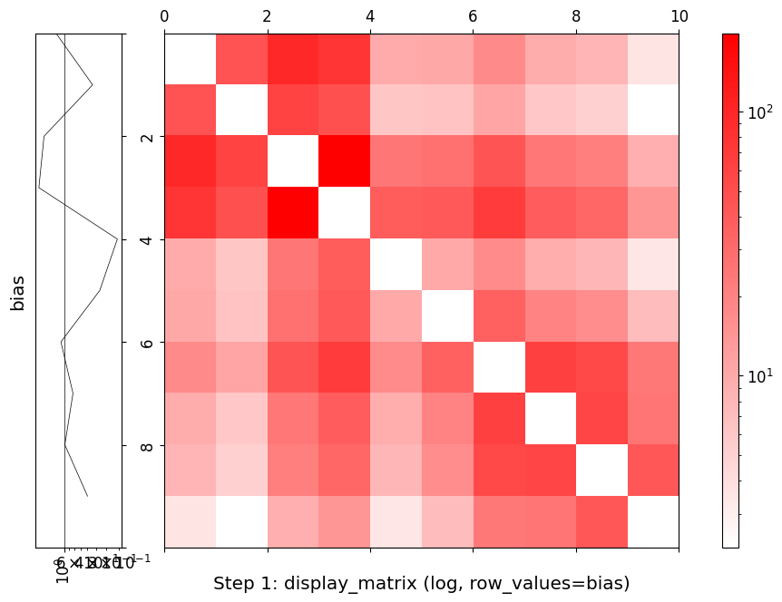
## Step 1: display_matrix with log=True and row_values for a per-bin value bar.

out1 = str(Path(ROOT) / 'notebooks' / 'tutorial_visualize_matrix.png')

try:
    display_matrix(
        matrix,
        log=True,
        title='Step 1: display_matrix (log, row_values=bias)',
        row_values=row_values,
        row_values_title='bias',
        row_values_log=True,
    )
    fig = plt.gcf()
    fig.savefig(out1, dpi=100, bbox_inches='tight')
    plt.close('all')
    print(f'Saved: {out1}')
except Exception as exc:
    plt.close('all')
    print(f'[skip] display_matrix failed: {exc!r}')
ipydisplay(ipyimage(filename=out1))
Saved: /home/adhisant/workspace/gunz-cm/notebooks/tutorial_visualize_matrix.png
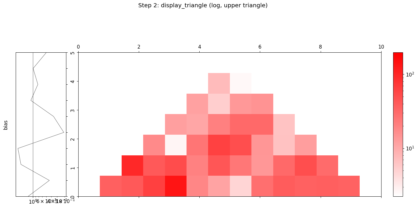
## Step 2: display_triangle renders only the upper triangle of a symmetric matrix
## with an optional values bar on the hypotenuse.

out2 = str(Path(ROOT) / 'notebooks' / 'tutorial_visualize_triangle.png')

try:
    display_triangle(
        matrix,
        log=True,
        title='Step 2: display_triangle (log, upper triangle)',
        values=row_values,
        values_log=True,
        values_title='bias',
    )
    fig = plt.gcf()
    fig.savefig(out2, dpi=100, bbox_inches='tight')
    plt.close('all')
    print(f'Saved: {out2}')
except Exception as exc:
    plt.close('all')
    print(f'[skip] display_triangle failed: {exc!r}')
ipydisplay(ipyimage(filename=out2))
Saved: /home/adhisant/workspace/gunz-cm/notebooks/tutorial_visualize_triangle.png
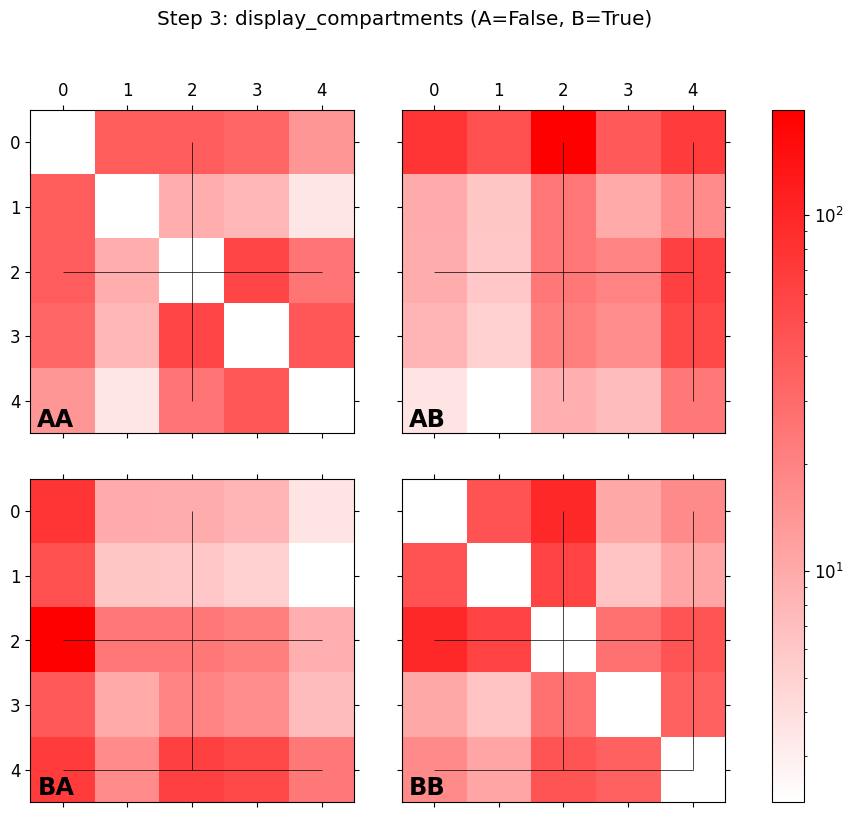
## Step 3: display_compartments partitions the matrix into the four A/A, A/B, B/A, B/B
## quadrants from a boolean compartment vector (A=False, B=True) and plots them in a 2x2 grid.

out3 = str(Path(ROOT) / 'notebooks' / 'tutorial_visualize_compartments.png')

try:
    display_compartments(
        matrix,
        compartments,
        log=True,
        title='Step 3: display_compartments (A=False, B=True)',
    )
    fig = plt.gcf()
    fig.savefig(out3, dpi=100, bbox_inches='tight')
    plt.close('all')
    print(f'Saved: {out3}')
except Exception as exc:
    plt.close('all')
    print(f'[skip] display_compartments failed: {exc!r}')
ipydisplay(ipyimage(filename=out3))
Saved: /home/adhisant/workspace/gunz-cm/notebooks/tutorial_visualize_compartments.png
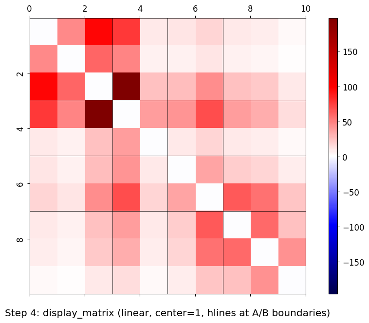
## Step 4: Common parameters - linear (log=False), divergent colormap centered at 1,
## and hlines/vlines marking A/B compartment boundaries.

boundaries = np.where(np.diff(compartments.astype(int)))[0] + 1
out4 = str(Path(ROOT) / 'notebooks' / 'tutorial_visualize_centered.png')

try:
    display_matrix(
        matrix,
        log=False,
        center=1,
        title='Step 4: display_matrix (linear, center=1, hlines at A/B boundaries)',
        hlines=boundaries,
        vlines=boundaries,
    )
    fig = plt.gcf()
    fig.savefig(out4, dpi=100, bbox_inches='tight')
    plt.close('all')
    print(f'Saved: {out4}')
    print(f'A/B boundaries drawn at indices: {boundaries.tolist()}')
except Exception as exc:
    plt.close('all')
    print(f'[skip] display_matrix (centered) failed: {exc!r}')
ipydisplay(ipyimage(filename=out4))
Saved: /home/adhisant/workspace/gunz-cm/notebooks/tutorial_visualize_centered.png
A/B boundaries drawn at indices: [3, 5, 7]
Summary#
In this tutorial you learned how to:
Build a synthetic Hi-C matrix with distance decay and visibility bias, plus a synthetic A/B compartment vector.
Render a full heatmap with
display_matrix(..., log=True, row_values=...)to attach a per-bin value bar.Render the upper triangle with
display_triangle(..., log=True, values=...)for symmetric matrices.Render the 2x2 A/B quadrant grid with
display_compartments(matrix, compartments, log=True).Switch to a divergent colormap with
display_matrix(..., log=False, center=1, hlines=..., vlines=...)and overlay reference lines at compartment boundaries.
All three helpers return a matplotlib figure that the caller saves to disk via plt.gcf().savefig(...) (or shows interactively with %matplotlib inline / widget). The same pattern works on real data: load a contact matrix with gunz_cm.loaders.load_cm_data(...) and pass coo_matrix(...).toarray() as the matrix argument.
Next steps:
tutorial_load_cooler.ipynb- loading a real.cool/.mcoolmatrixtutorial_compartments.ipynb- computing A/B compartments from a real matrixtutorial_filter_normalize.ipynb- filtering and balancing before display
## Cleanup - confirm the four PNGs were written next to the notebook.

import os

saved = [
    str(Path(ROOT) / 'notebooks' / 'tutorial_visualize_matrix.png'),
    str(Path(ROOT) / 'notebooks' / 'tutorial_visualize_triangle.png'),
    str(Path(ROOT) / 'notebooks' / 'tutorial_visualize_compartments.png'),
    str(Path(ROOT) / 'notebooks' / 'tutorial_visualize_centered.png'),
]
for p in saved:
    if os.path.exists(p):
        size_kb = os.path.getsize(p) / 1024.0
        print(f'kept:   {p}  ({size_kb:.1f} KB)')
    else:
        print(f'missing: {p}')
plt.close('all')
kept:   /home/adhisant/workspace/gunz-cm/notebooks/tutorial_visualize_matrix.png  (30.4 KB)
kept:   /home/adhisant/workspace/gunz-cm/notebooks/tutorial_visualize_triangle.png  (35.5 KB)
kept:   /home/adhisant/workspace/gunz-cm/notebooks/tutorial_visualize_compartments.png  (27.6 KB)
kept:   /home/adhisant/workspace/gunz-cm/notebooks/tutorial_visualize_centered.png  (25.6 KB)