Tutorial: Load COOL / MCOOL contact matrix data#
This tutorial walks through loading a Hi-C contact matrix from a .cool or .mcool (multi-resolution) file using the gunz_cm.loaders API. You will learn how to:
Create a synthetic multi-resolution
.mcoolfile inline withcooler.create_cooler+cooler.zoomify_coolerQuery available resolutions in a multi-resolution cooler
Query chromosome information (names, lengths)
Load a contact matrix at a specific resolution and region in your preferred output format
Iterate over all available resolutions in a
.mcooland compare shapes
The worked examples use a synthetic .mcool file (created inline below) because it loads reliably with the current gunz_cm build. The API surface for .cool and .mcool is identical at the load_cm_data(...) call site — the difference is just the set of resolutions you can choose from.
Initialization#
Set auto-reload so edits to the source code are picked up without restarting the kernel.
%load_ext autoreload
%autoreload 2
Add the repository root to sys.path so the gunz_cm package can be imported.
import sys
from git.repo import Repo

repo = Repo('.', search_parent_directories=True)
ROOT = repo.working_tree_dir

assert isinstance(ROOT, str)
sys.path.append(ROOT)
print(f'Repo root: {ROOT}')
Repo root: /home/adhisant/workspace/gunz-cm
Imports#
import tempfile
from pathlib import Path

import pandas as pd
import numpy as np

import cooler

from gunz_cm.loaders import (
    load_cm_data,
    get_resolutions,
    get_chrom_infos,
)
from gunz_cm.consts import DataStructure
Create a synthetic multi-resolution .mcool file#
We build a synthetic .mcool (multi-resolution cooler) in two steps:
cooler.create_coolerwrites the base resolution (finest bin size).cooler.zoomify_coolerrecursively aggregates bins to produce coarser resolutions, all stored inside the same.mcoolfile underresolutions/<r>.
Zoomify is constrained: every target resolution must be an integer multiple of the base (finest) resolution. We start from a 100 kb base and generate three resolutions: 100 kb, 1 Mb, and 5 Mb.
For a real .mcool file, replace this with:
fpath = '/path/to/your/data.mcool'
and skip the file-creation step. The load_cm_data(...) API is identical.
tmpdir = tempfile.mkdtemp(prefix='gunz_cm_tutorial_')
fpath = str(Path(tmpdir) / 'synthetic.mcool')

# Base resolution: 100 kb. chr1 -> 50 bins, chr2 -> 40 bins.
base_res = 100_000
n1, n2 = 50, 40
starts1 = np.arange(n1) * base_res
starts2 = np.arange(n2) * base_res
bins = pd.DataFrame({
    'chrom': ['chr1'] * n1 + ['chr2'] * n2,
    'start': list(starts1) + list(starts2),
    'end':   list(starts1 + base_res) + list(starts2 + base_res),
})

# Synthetic pixel weights: exponentially decaying with genomic distance.
n = len(bins)
rows, cols, counts = [], [], []
for i in range(n):
    for j in range(i, n):
        dist = abs(bins['start'].iloc[i] - bins['start'].iloc[j])
        weight = 100.0 * np.exp(-dist / 2_000_000.0)
        rows.append(i)
        cols.append(j)
        counts.append(weight)
pixels = pd.DataFrame({'bin1_id': rows, 'bin2_id': cols, 'count': counts})

# Step 1: write base 100 kb cooler.
base_fpath = str(Path(tmpdir) / 'base_100kb.cool')
cooler.create_cooler(base_fpath, bins, pixels, symmetric_upper=True, mode='w')
print(f'Base resolution: {base_res:,} bp ({len(bins)} bins, {len(pixels)} non-zero pixels)')

# Step 2: zoomify into a multi-resolution .mcool.
# Target resolutions must be integer multiples of the base resolution (100 kb).
target_resolutions = [100_000, 1_000_000, 5_000_000]
cooler.zoomify_cooler(
    base_uris=base_fpath,
    outfile=fpath,
    resolutions=target_resolutions,
    chunksize=100,
    nproc=1,
)
print(f'Zoomified .mcool: {fpath} ({Path(fpath).stat().st_size} bytes)')
print(f'  Resolutions stored: {target_resolutions}')
Base resolution: 100,000 bp (90 bins, 4095 non-zero pixels)
Zoomified .mcool: /tmp/gunz_cm_tutorial_2ijeg_yq/synthetic.mcool (122281 bytes)
  Resolutions stored: [100000, 1000000, 5000000]
Step 1: Query the file’s metadata#
Before loading data, you usually want to know what resolutions and chromosomes are available. gunz_cm.loaders exposes metadata-query functions that work for both .cool and .mcool. The key difference: for a .mcool file, get_resolutions returns a list of all available resolutions; for a single-resolution .cool file, it raises LoaderError (covered in tutorial_load_hic.ipynb).
Available resolutions#
resolutions = get_resolutions(fpath)
print(f'Available resolutions: {sorted(resolutions)}')
print(f'Sorted ascending: {sorted(resolutions)}')
print(f'  - finest (base):   {min(resolutions):,} bp')
print(f'  - coarsest:        {max(resolutions):,} bp')
print(f'  - number of zoom levels: {len(resolutions)}')
Available resolutions: [100000, 1000000, 5000000]
Sorted ascending: [100000, 1000000, 5000000]
  - finest (base):   100,000 bp
  - coarsest:        5,000,000 bp
  - number of zoom levels: 3


/tmp/ipykernel_2697605/2254348678.py:1: DeprecationWarning: get_resolutions() is deprecated and will be removed in v2.13.0. Use get_bin_size_bps() instead.
  resolutions = get_resolutions(fpath)
get_resolutions is the canonical way to discover which zoom levels are embedded in a .mcool. Internally it reads the resolutions/ group of the HDF5 file.
Chromosome information#
chroms_info = get_chrom_infos(fpath)
print('Chromosome info (dict):')
for chrom, info in chroms_info.items():
    print(f'  {chrom}: {info}')
Chromosome info (dict):
  chr1: {'name': 'chr1', 'length': 5000000}
  chr2: {'name': 'chr2', 'length': 4000000}
The result is a dict[str, dict[str, str | int]] mapping chromosome name to its info (typically name, length, offset). For real .mcool files generated by cooler, the chrom names follow the source assembly’s native convention (typically chr1, chr2, …).
Step 2: Load a contact matrix at a specific resolution#
Use load_cm_data(...) to load a region of the matrix. The required arguments are the file path and the resolution; region1 and region2 specify the genomic interval.
The default return type is pd.DataFrame with columns [row_ids, col_ids, counts]. You can request other formats via the output_format parameter.
# Pick a resolution from the list returned by get_resolutions().
resolutions = sorted(get_resolutions(fpath))
chosen = 1_000_000
assert chosen in resolutions, f'{chosen} not in {resolutions}'

cm_df = load_cm_data(
    fpath=fpath,
    bin_size_bp=chosen,
    region1='chr1',
    region2='chr1',
    balancing=None,  # raw counts
    output_format=DataStructure.DF,
)
print(f'Loading at {chosen:,} bp (chr1:chr1):')
print('  Return type:', type(cm_df).__name__)
print('  Shape:', cm_df.shape)
print('  Columns:', list(cm_df.columns))
print()
print('Head:')
print(cm_df.head().to_string(index=False))
Loading at 1,000,000 bp (chr1:chr1):
  Return type: DataFrame
  Shape: (25, 3)
  Columns: ['row_ids', 'col_ids', 'counts']

Head:
 row_ids  col_ids  counts
       0        0    4751
       0        1    6137
       0        2    3693
       0        3    2235
       0        4    1334


/tmp/ipykernel_2697605/2338234655.py:2: DeprecationWarning: get_resolutions() is deprecated and will be removed in v2.13.0. Use get_bin_size_bps() instead.
  resolutions = sorted(get_resolutions(fpath))
Request a sparse matrix output#
cm_coo = load_cm_data(
    fpath=fpath,
    bin_size_bp=1_000_000,
    region1='chr1',
    region2='chr1',
    output_format=DataStructure.COO,
)
print('COO type:', type(cm_coo).__name__)
print('Shape:', cm_coo.shape, 'nnz:', cm_coo.nnz)

dense_1mb = cm_coo.toarray()
print('Dense shape:', dense_1mb.shape)
print('Sum of all counts:', dense_1mb.sum())
COO type: coo_matrix
Shape: (5, 5) nnz: 25
Dense shape: (5, 5)
Sum of all counts: 106617
Switch to a different resolution#
# Load the same region at the finest (base) resolution. The shape is 10x larger per axis.
cm_fine = load_cm_data(
    fpath=fpath,
    bin_size_bp=100_000,
    region1='chr1',
    region2='chr1',
    output_format=DataStructure.COO,
)
dense_100kb = cm_fine.toarray()
print(f'Loading the same region at 100,000 bp:')
print(f'  Shape: {cm_fine.toarray().sum().item()}...') if False else None  # noqa
print(f'  Shape: {dense_100kb.shape[0]*dense_100kb.shape[1]} cells = {cm_fine.nnz} non-zero, dense {dense_100kb.shape}')
print(f'  First few rows of the COO coordinate DataFrame view:')
cm_fine_df = load_cm_data(
    fpath=fpath,
    bin_size_bp=100_000,
    region1='chr1',
    region2='chr1',
    output_format=DataStructure.DF,
)
print(cm_fine_df.head().to_string(index=False))
Loading the same region at 100,000 bp:
  Shape: 2500 cells = 2500 non-zero, dense (50, 50)
  First few rows of the COO coordinate DataFrame view:
 row_ids  col_ids  counts
       0        0     100
       0        1      95
       0        2      90
       0        3      86
       0        4      81
Step 3: Iterate over all resolutions#
A common workflow is to load the same region at every available resolution and compare shapes / total counts. This is the recommended pattern for picking the right resolution for downstream analysis (e.g. TAD calling, compartment analysis).
print('chr1:chr1 across all resolutions:')
print(f'  {"resolution":>13}  {"shape":>7}  {"nnz":>6}  {"sum(counts)":>12}')
print(f'  {"-"*13}  {"-"*7}  {"-"*6}  {"-"*12}')
for res in sorted(get_resolutions(fpath)):
    cm = load_cm_data(
        fpath=fpath,
        bin_size_bp=res,
        region1='chr1',
        region2='chr1',
        output_format=DataStructure.COO,
    )
    dense = cm.toarray()
    print(f'  {res:>13,}  {cm.shape[0]}x{cm.shape[1]:<3}  {cm.nnz:>6}  {dense.sum():>12.2e}')
chr1:chr1 across all resolutions:
     resolution    shape     nnz   sum(counts)
  -------------  -------  ------  ------------
        100,000  50x50     2500      1.25e+05
      1,000,000  5x5        25      1.07e+05
      5,000,000  1x1         1      6.52e+04


/tmp/ipykernel_2697605/2282641961.py:4: DeprecationWarning: get_resolutions() is deprecated and will be removed in v2.13.0. Use get_bin_size_bps() instead.
  for res in sorted(get_resolutions(fpath)):
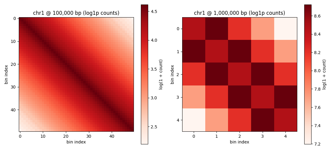
Notice how the matrix shrinks as resolution coarsens: 5 Mb resolution collapses the entire 5 Mb chr1 into a single bin. The total sum(counts) decreases as well because the diagonal and near-diagonal short-range interactions get merged into single bins.
Step 4: v2.8.0 — Chromosome name normalization#
Since v2.8.0, you can pass chromosome names in either UCSC (chr1) or Ensembl (1) form. The facade normalizes them to match the file’s native convention automatically.
# Synthetic file uses 'chr1' (UCSC). Try passing '1' (Ensembl).
try:
    cm_bare = load_cm_data(fpath=fpath, bin_size_bp=1_000_000, region1='1', region2='1')
    print('Loaded with Ensembl-style input ("1") even though file uses UCSC ("chr1")')
    print(f'  - rows: {len(cm_bare)}')
except Exception as e:
    print(f'Error: {type(e).__name__}: {e}')
Loaded with Ensembl-style input ("1") even though file uses UCSC ("chr1")
  - rows: 25
Not normalized (out of scope per the design):
Mitochondrial chroms:
chrM/MT/MRandom contigs:
chr1_KI270706v1_randomGenBank accessions
Case variants:
Chr1≠chr1
Use get_chrom_infos(fpath) to see the actual file chrom names.
Step 5: Visualize side-by-side at two resolutions#
import matplotlib
from IPython.display import display as ipydisplay
matplotlib.use('Agg')  # non-interactive backend for CI / headless environments
import matplotlib.pyplot as plt
from IPython.display import Image as ipyimage, display as ipydisplay

fig, axes = plt.subplots(1, 2, figsize=(11, 5))
for ax, res, dense in [
    (axes[0], 100_000, dense_100kb),
    (axes[1], 1_000_000, dense_1mb),
]:
    im = ax.imshow(np.log1p(dense), cmap='Reds', aspect='equal')
    ax.set_title(f'chr1 @ {res:,} bp (log1p counts)')
    ax.set_xlabel('bin index')
    ax.set_ylabel('bin index')
    fig.colorbar(im, ax=ax, label='log(1 + count)')
plt.tight_layout()
out_png = str(Path(tmpdir) / 'contact_map_two_resolutions.png')
plt.savefig(out_png, dpi=100)
print(f'Saved: {out_png}')
print(f'  - 100,000 bp panel: {dense_100kb.shape} ({int((dense_100kb > 0).sum())} non-zero)')
print(f'  - 1,000,000 bp panel: {dense_1mb.shape} ({int((dense_1mb > 0).sum())} non-zero)')
ipydisplay(ipyimage(filename=out_png))
Saved: /tmp/gunz_cm_tutorial_2ijeg_yq/contact_map_two_resolutions.png
  - 100,000 bp panel: (50, 50) (2500 non-zero)
  - 1,000,000 bp panel: (5, 5) (25 non-zero)
Summary#
In this tutorial you learned how to:
Build a synthetic multi-resolution
.mcoolfile by chainingcooler.create_cooler(base resolution) withcooler.zoomify_cooler(recursive coarsening).Query file metadata with
get_resolutions(returns the full list of zoom levels) andget_chrom_infos(chrom names + lengths).Load a contact matrix at a chosen resolution with
load_cm_data(file, resolution, region1, region2, balancing, output_format).Iterate over all resolutions in a
.mcooland compare matrix shapes / total counts to pick the right zoom level for downstream analysis.Choose the output format:
DataStructure.DF(default),DataStructure.COO(sparse), or others.Use v2.8.0 chrom name normalization — pass
chr1or1, the facade normalizes for you.Visualize two resolutions side-by-side via matplotlib.
Next steps:
tutorial_load_hic.ipynb—.hicfile loading (Juicer / HiC-Pro / hictkpy)tutorial_balance_kr.ipynb— applying KR / VC / ICE balancingtutorial_3d_reconstruction.ipynb— going from 2D contact matrix to 3D structure
Cleanup#
import shutil
shutil.rmtree(tmpdir, ignore_errors=True)
print(f'Removed: {tmpdir}')
Removed: /tmp/gunz_cm_tutorial_2ijeg_yq