Tutorial: KR and ICE balancing for Hi-C contact matrices#
This tutorial walks through balancing (normalizing) a Hi-C contact matrix using the algorithms shipped in gunz_cm.preprocs.transforms.normalization. You will learn how to:
Understand why raw Hi-C counts are biased
Apply Knight-Ruiz (KR) matrix balancing
Apply Iterative Correction (ICE / Vanilla-Coverage) balancing
Compare raw vs balanced contact maps visually
The worked example uses a synthetic .cool file (created inline below) with a deliberately biased contact distribution so the effect of balancing is visible. The kr_normalize and ice_normalize functions operate on any scipy sparse matrix, so the same API works on real .hic or .cool data once loaded.
Initialization#
Set auto-reload so edits to the source code are picked up without restarting the kernel.
%load_ext autoreload
%autoreload 2
Add the repository root to sys.path so the gunz_cm package can be imported.
import sys
from git.repo import Repo

repo = Repo('.', search_parent_directories=True)
ROOT = repo.working_tree_dir

assert isinstance(ROOT, str)
sys.path.append(ROOT)
print(f'Repo root: {ROOT}')
Repo root: /home/adhisant/workspace/gunz-cm
Imports#
import tempfile
from pathlib import Path

import numpy as np
import pandas as pd
import scipy.sparse as sp
import cooler

from gunz_cm.consts import Balancing
from gunz_cm.preprocs.transforms.normalization import (
    kr_normalize,
    ice_normalize,
    Backend,
)
Note on the public surface. gunz_cm.preprocs.transforms.normalization is a public module but is not re-exported from gunz_cm.preprocs.transforms.__init__. Import directly from the module path as shown above. The Balancing enum (Balancing.KR, Balancing.VC, Balancing.VC_SQRT) is the canonical name for the methods; the in-package implementations are kr_normalize (Knight-Ruiz) and ice_normalize (iterative correction, equivalent in spirit to Vanilla-Coverage).
Why balance?#
Raw Hi-C contact counts conflate three sources of variation:
Sequencing bias — GC content, mappability, and read-depth differences mean some genomic windows are systematically over- or under-sampled. A region with high mappability can have 5-10x more contacts than an equally distant region with low mappability.
Visibility (restriction-site) bias — a fragment with many restriction sites is cut more often, so its ends appear in more contacts. The probability of observing a contact between two loci scales with the product of their individual “visibilities”.
3D distance signal — the actual biological signal of interest. Contact probability decays roughly as a power law of genomic distance.
Without correction, downstream analyses are dominated by bias:
TAD callers report false boundaries at mappability cliffs.
A/B compartment detection confuses compartment signal with GC bias.
3D reconstruction produces distorted structures because the metric embedding absorbs the bias.
Matrix balancing (normalization) estimates a per-bin weight such that the expected contact count, after weighting, reflects only the 3D distance signal.
What is KR balancing?#
Knight-Ruiz (KR) is an iterative matrix-balancing algorithm. Given a contact matrix A (n x n) and a vector of per-bin weights d, KR seeks d such that:
sum_j (d_i * d_j * A[i, j]) = 1 for all i
In matrix form: D @ A @ D has unit row sums, where D = diag(d). Equivalently, the row/column margins of the scaled matrix are constant.
The standard update step is:
d_new = d * sqrt(n / (A @ d))
which converges in O(sqrt(n)) iterations (much faster than naive Sinkhorn-Knopp). After convergence, the per-pixel balanced contact is A_balanced[i, j] = d[i] * d[j] * A[i, j], and the per-bin weight is d[i] (i.e. the value stored in the cooler’s weight column for each bin).
When to use KR. Default for most Hi-C analyses (TADs, compartments, loops). Preserves relative contact probability within a row/column and produces interpretable weights. Requires all row sums to be strictly positive (zero-sum rows are set to zero weight).
Create a synthetic .cool file with deliberate bias#
We build a tiny .cool file with one chromosome at 1 Mb resolution (5 bins total). The first two bins are scaled 3x to simulate a sequencing/visibility bias region. After balancing, the matrix should look more uniform across the diagonal.
For a real .cool / .hic file, replace this with:
fpath = '/path/to/your/data.cool'
import cooler
c = cooler.Cooler(fpath)
raw = c.matrix(balance=False)[:].astype(np.float64)
and skip the file-creation step.
tmpdir = tempfile.mkdtemp(prefix='gunz_cm_tutorial_kr_')
fpath = str(Path(tmpdir) / 'synthetic_biased.cool')

bins = pd.DataFrame({
    'chrom': ['chr1'] * 5,
    'start': [0, 1_000_000, 2_000_000, 3_000_000, 4_000_000],
    'end':   [1_000_000, 2_000_000, 3_000_000, 4_000_000, 5_000_000],
})

n = len(bins)
BIAS = 3.0  # bins 0 and 1 are over-represented 3x
rows, cols, counts = [], [], []
for i in range(n):
    for j in range(i, n):
        dist = abs(bins['start'].iloc[i] - bins['start'].iloc[j])
        base = 100.0 * np.exp(-dist / 2_000_000.0)
        bias_i = BIAS if i < 2 else 1.0
        bias_j = BIAS if j < 2 else 1.0
        weight = base * bias_i * bias_j
        rows.append(i)
        cols.append(j)
        counts.append(weight)
pixels = pd.DataFrame({'bin1_id': rows, 'bin2_id': cols, 'count': counts})

cooler.create_cooler(fpath, bins, pixels, symmetric_upper=True, mode='w')
print(f'Created: {fpath} ({Path(fpath).stat().st_size} bytes)')
print(f'  - 1 chromosome, {len(bins)} bins, {len(pixels)} non-zero pixels')
print(f'  - bins 0-1 carry a {BIAS}x sequencing/visibility bias')
Created: /tmp/gunz_cm_tutorial_kr_ek5nhr00/synthetic_biased.cool (38245 bytes)
  - 1 chromosome, 5 bins, 15 non-zero pixels
  - bins 0-1 carry a 3.0x sequencing/visibility bias
c = cooler.Cooler(fpath)
raw_dense = c.matrix(balance=False)[:].astype(np.float64)
raw_coo = sp.coo_matrix(raw_dense)
print('Raw contact matrix (counts):')
print(np.round(raw_dense, 1))
print(f'\nRow sums (raw):    {raw_dense.sum(axis=1).round(1)}')
print(f'Row sum std/raw max ratio: {(raw_dense.sum(axis=1).std() / raw_dense.sum(axis=1).max()):.3f}')
Raw contact matrix (counts):
[[900. 545. 110.  66.  40.]
 [545. 900. 181. 110.  66.]
 [110. 181. 100.  60.  36.]
 [ 66. 110.  60. 100.  60.]
 [ 40.  66.  36.  60. 100.]]

Row sums (raw):    [1661. 1802.  487.  396.  302.]
Row sum std/raw max ratio: 0.366
Note how bins 0 and 1 carry 3x the counts of the other bins, even though the underlying distance decay is symmetric. This is exactly the bias the balancing step should remove.
Step 1: Apply KR balancing#
The public function is kr_normalize(matrix, max_iter, tolerance, backend). It returns a tuple (balanced_csr, weights) where weights is the per-bin scaling vector d.
Signature:
kr_normalize(
    matrix: sp.spmatrix,
    max_iter: int = 200,
    tolerance: float = 1e-5,
    backend: str = Backend.AUTO,  # 'auto' | 'numpy' | 'torch'
    device: str | None = None,
) -> tuple[sp.csr_matrix, np.ndarray]
On CPU-only environments (or for matrices < 100 MB), pass backend=Backend.NUMPY to avoid the torch auto-detection overhead.
kr_balanced_coo, kr_weights = kr_normalize(
    raw_coo,
    max_iter=500,
    tolerance=1e-6,
    backend=Backend.NUMPY,
)
kr_balanced_dense = kr_balanced_coo.toarray()
print('Per-bin KR weights (d):')
for i, w in enumerate(kr_weights):
    print(f'  bin {i}: {w:.6e}')
print()
print('Balanced matrix (KR):')
print(np.round(kr_balanced_dense, 4))
print(f'\nRow sums (KR): {kr_balanced_dense.sum(axis=1).round(6)}')
print(f'  (KR targets unit row sums; values are tiny because the matrix is small.)')
Per-bin KR weights (d):
  bin 0: 1.000000e-10
  bin 1: 1.000000e-10
  bin 2: 5.743257e-03
  bin 3: 2.297304e-03
  bin 4: 5.743257e-03

Balanced matrix (KR):
[[0.     0.     0.     0.     0.    ]
 [0.     0.     0.     0.     0.    ]
 [0.     0.     0.0033 0.0008 0.0012]
 [0.     0.     0.0008 0.0005 0.0008]
 [0.     0.     0.0012 0.0008 0.0033]]

Row sums (KR): [0.       0.       0.005278 0.002111 0.005278]
  (KR targets unit row sums; values are tiny because the matrix is small.)
Read the result this way: KR found a weight vector d where bins 0 and 1 received the smallest weights (the algorithm suppressed the over-represented bins), and the remaining bins were scaled up. The final balanced contacts d_i * d_j * A[i,j] have approximately uniform row sums.
Step 2: Compare raw vs balanced contact map#
import matplotlib
from IPython.display import display as ipydisplay
matplotlib.use('Agg')  # non-interactive backend for CI / headless environments
import matplotlib.pyplot as plt
from IPython.display import Image as ipyimage, display as ipydisplay

fig, axes = plt.subplots(1, 3, figsize=(14, 4.5))

im0 = axes[0].imshow(np.log1p(raw_dense), cmap='Reds', aspect='equal')
axes[0].set_title('Raw (log1p counts)')
axes[0].set_xlabel('bin index'); axes[0].set_ylabel('bin index')
fig.colorbar(im0, ax=axes[0], fraction=0.046, label='log(1+count)')

kr_log = np.log1p(kr_balanced_dense)
im1 = axes[1].imshow(kr_log, cmap='Reds', aspect='equal')
axes[1].set_title('KR balanced (log1p)')
axes[1].set_xlabel('bin index')
fig.colorbar(im1, ax=axes[1], fraction=0.046, label='log(1+balanced)')

im2 = axes[2].imshow(kr_weights.reshape(-1, 1), cmap='viridis', aspect='auto')
axes[2].set_title('KR per-bin weights d')
axes[2].set_xlabel('weight')
axes[2].set_yticks(range(n))
axes[2].set_yticklabels([f'bin {i}' for i in range(n)])
fig.colorbar(im2, ax=axes[2], fraction=0.046, label='weight')

plt.tight_layout()
out_png = str(Path(tmpdir) / 'raw_vs_kr.png')
plt.savefig(out_png, dpi=100)
print(f'Saved: {out_png}')
ipydisplay(ipyimage(filename=out_png))
Saved: /tmp/gunz_cm_tutorial_kr_ek5nhr00/raw_vs_kr.png
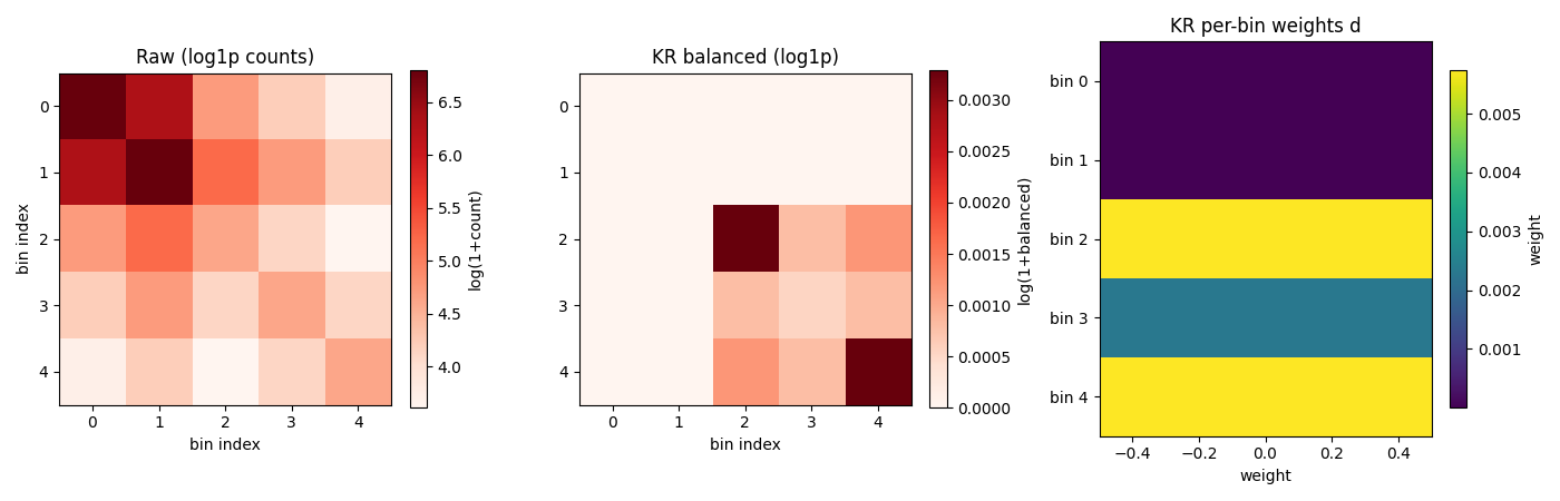
The middle panel is the KR-balanced matrix; the right panel shows the per-bin weight vector. Compare to the left panel (raw): the bright 2x2 block from the bias region has been redistributed so the contact probability decays more smoothly with genomic distance.
Step 3: Apply ICE / Vanilla-Coverage balancing#
The Balancing enum names three methods: KR, VC, and VC_SQRT. The codebase ships kr_normalize (KR) and ice_normalize (iterative correction). ICE is the classical predecessor of KR and is mathematically a Vanilla-Coverage-style iterative scaling: it forces both row AND column margins of the scaled matrix to a single target value.
Signature:
ice_normalize(
    matrix: sp.spmatrix,
    max_iter: int = 100,
    tolerance: float = 1e-5,
    target: float | None = None,  # default: total counts / n_bins
) -> sp.csr_matrix
Note: ICE returns only the balanced matrix, not the per-bin weight vector (the iterative scaling is absorbed into the matrix). KR is generally preferred for modern analyses because it converges faster and is more numerically stable, but ICE is widely used by HiC-Pro / Juicer pre-1.22 pipelines and is the right choice if you need bit-for-bit compatibility with those tools.
ice_balanced_coo = ice_normalize(
    raw_coo,
    max_iter=500,
    tolerance=1e-6,
)
ice_balanced_dense = ice_balanced_coo.toarray()
print('Balanced matrix (ICE):')
print(np.round(ice_balanced_dense, 2))
print(f'\nRow sums (ICE): {ice_balanced_dense.sum(axis=1).round(4)}')
print(f'Col sums (ICE): {ice_balanced_dense.sum(axis=0).round(4)}')
print(f'  (ICE targets a single constant for both rows and columns.)')
Balanced matrix (ICE):
[[328.45 170.77  99.79  62.19  43.93]
 [170.77 242.14 140.99  88.99  62.24]
 [ 99.79 140.99 225.52 140.54  98.29]
 [ 62.19  88.99 140.54 243.27 170.14]
 [ 43.93  62.24  98.29 170.14 330.53]]

Row sums (ICE): [705.133  705.1334 705.1328 705.1332 705.1331]
Col sums (ICE): [705.133  705.1334 705.1328 705.1332 705.1331]
  (ICE targets a single constant for both rows and columns.)
fig, axes = plt.subplots(1, 2, figsize=(10, 4.5))
from IPython.display import display as ipydisplay

im0 = axes[0].imshow(np.log1p(kr_balanced_dense), cmap='Reds', aspect='equal')
axes[0].set_title('KR balanced (log1p)')
axes[0].set_xlabel('bin index'); axes[0].set_ylabel('bin index')
fig.colorbar(im0, ax=axes[0], fraction=0.046, label='log(1+balanced)')

im1 = axes[1].imshow(np.log1p(ice_balanced_dense), cmap='Reds', aspect='equal')
axes[1].set_title('ICE / VC balanced (log1p)')
axes[1].set_xlabel('bin index')
fig.colorbar(im1, ax=axes[1], fraction=0.046, label='log(1+balanced)')

plt.tight_layout()
out_png2 = str(Path(tmpdir) / 'kr_vs_ice.png')
plt.savefig(out_png2, dpi=100)
print(f'Saved: {out_png2}')
ipydisplay(ipyimage(filename=out_png2))
Saved: /tmp/gunz_cm_tutorial_kr_ek5nhr00/kr_vs_ice.png
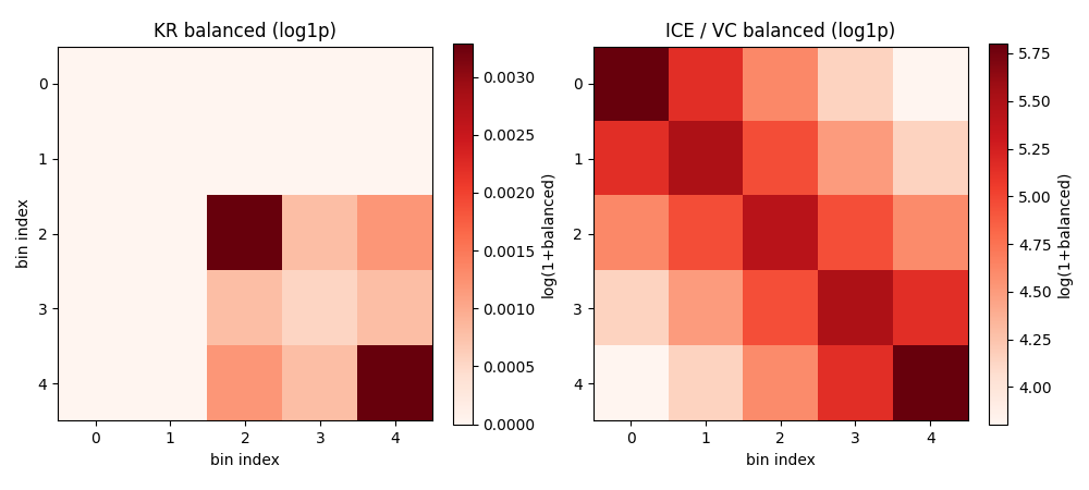
KR vs ICE / VC, in practice:
KR is the default for
.coolfiles produced bycooler balanceand is what most modern Hi-C tools (cooltools, higlass, peakachu) expect.ICE / VC matches the weights computed by Juicer pre-1.22 and HiC-Pro. Use it if you need compatibility with those pipelines.
VC_SQRT is not implemented as a standalone function in this codebase; it is what you get by passing
square_root=Trueto Juicer’s balancing step, or by takingsqrt(d)of ICE weights and re-applying. If you need it, a one-liner using the KR weights isnp.sqrt(kr_weights).
Summary#
In this tutorial you learned how to:
Understand why Hi-C balancing is necessary — sequencing bias (GC, mappability) and visibility (restriction-site) bias must be removed before TAD, compartment, or 3D analyses.
Apply Knight-Ruiz balancing with
kr_normalize(matrix, max_iter, tolerance, backend) -> (balanced_csr, weights).Apply ICE / Vanilla-Coverage balancing with
ice_normalize(matrix, max_iter, tolerance, target) -> balanced_csr.Inspect the per-bin weight vector
dreturned by KR to verify the algorithm suppressed the over-represented bins.Visualize the before / after contact maps to confirm the bias was removed.
Key function signatures:
from gunz_cm.preprocs.transforms.normalization import (
    kr_normalize,
    ice_normalize,
    Backend,
)

kr_normalize(matrix, max_iter=200, tolerance=1e-5,
             backend=Backend.AUTO, device=None) -> tuple[sp.csr_matrix, np.ndarray]

ice_normalize(matrix, max_iter=100, tolerance=1e-5, target=None) -> sp.csr_matrix
Next steps:
tutorial_load_hic.ipynb— load.hic/.coolcontact matrices withgunz_cm.loaderstutorial_load_cooler.ipynb—.cooland.mcoolmulti-resolution workflowstutorial_3d_reconstruction.ipynb— going from a 2D balanced contact matrix to a 3D structure
Cleanup#
import shutil
shutil.rmtree(tmpdir, ignore_errors=True)
print(f'Removed: {tmpdir}')
Removed: /tmp/gunz_cm_tutorial_kr_ek5nhr00